GIS3015 - Module 11 - 3D Mapping

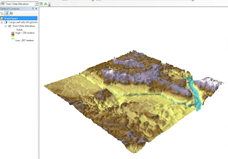
Figure 1: Vertical Exaggeration of Twin Cities Elevation (MN)

In this week's Module, 3D Mapping, we first worked through an ESRI Training Module on 3D Visualization Techniques Using ArcGIS.  This training module introduced new terms in addition to new techniques.   We learned about Triangulated Irregular Networks (TINs), Terrain Datasets, and Multipatches.  The primary focus was working with 3D features, discrete geographic features such as buildings, rivers, and wells that can be found on or beneath a surface.  We used ArcScene to display 2D features in a 3D perspective.  The first portion of the training taught us how to navigate within ArcScene and view 3D data and how to use the Attribute Table's Shape field to determine if our data was a 3D feature class.  Next, we learned how to set Base Heights for raster data which are set to  0 by default.   Lastly, we learned techniques that enhance 3D views.  In Figure 1, we changed the visual effect of raster elevation data for the Twin Cities of Minnesota by exaggerating the differences in elevation values.   The "exaggeration" technique does not alter the measured values but changes their appearance.  A negative exaggeration has the effect of "inverting" the data's appearance.  By changing "illumination" values and background colors you can alter the appearance of data.   Changes to the appearance of the sun's light (angle or altitude) has the effect of emphasizing or reducing variations seen in the 3D surface.  The use of a background color can make a 3D layer "pop" or appear to float or provide geographic reference (sky, horizon, water body).

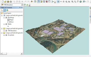Figure 2: Extrusion Of Buildings And Wells Using Elevation and Depth Values

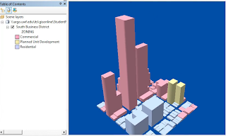Figure 3: Extrusion Of Parcels in Manhattan, Kansas Using Property Values

In Figure 2, we used the "extrusion" technique to extend features above and below the surface.   Buildings were extruded above the surface using their Height value and Wells were extruded below the surface using their Depth value.  Because wells appeared as flat points on the surface we applied an offset value to raise them slightly above the surface.  The "air photo" or picture layer in this figure was "draped" over the underlying elevation TIN layer, by setting the photo's base height to the elevation values of the TIN.

In Figure 3, we showed that z-values do not have to always represent height.  In this example, building parcels in Manhatten, Kansas were extruded based on their property value attribute.  Properties with a higher total value were extruded more than lower valued properties.  Sometimes, z-values may not be proportional to their x,y values.   In this example we had to also apply vertical exaggeration to the features so they would appear proportionally.

After completing the ESRI training course we moved on to our UWF exercise.  Using instructions and data provided by our professor and ArcGIS statistical tools we created sample points for 343 buildings in Boston.   With these points we performed calculations and determined a mean height for each building which represented our z-value.  The z-values were used to extrude the buildings in Boston.  We exported our extruded buildings data to create a layer and then converted that layer to a KML file.  Finally, we viewed our KML file in Google Earth as seen below in Figure 4.  The extruded buildings in Boston enable the viewer to visually focus on a specific area and view the buildings from different perspectives (above, street level, from different directions) as well as compare building heights relatively easily.

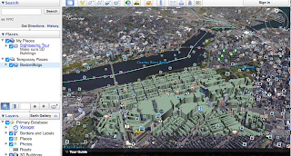Figure 4: Extruded Buildings In Boston Displayed Via Google Earth

Lastly, we took another look at Charles Minard's famous map of Napoleon's Russian Campaign of 1812 and compared it with Kenneth Field's and Nathan Shepherd's 3D version.  I really enjoyed this lab and some of the discussion posts by a classmate about Space Archeology.