GIS4043 - Week 5 - Projections Part 1

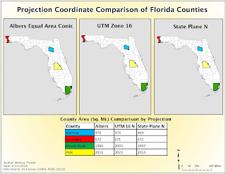
In this week's lab assignment we were tasked to learn about different projected coordinate systems and apply them to the same data set of Florida counties.  Using different projections we were able to see how differently the same data was displayed.    We learned how to use different Data Management Tools in the Arc Toolbox or via Search, specifically the Project Tool and the Project Raster Tool.

The Florida Counties data layer was originally projected in Albers Conical Equal Area projection.  An "Albers" layer was created in our Projection Comparison Map.  Then we used the Project Tool to create two new layers with new projection system.   The first new layer used the UTM 16N projection and the second new layer used the State Plane N (for Florida in US Feet) projection.   Each newly created layer was placed in a new data frame.   Now our Map contained three data frames with the same data set used to create three different projected layers.  Next we ordered the data displayed in each respective attribute table by County in alphabetical order.   We then added a new field and had it display the Area for each county in square miles.   From the attribute table we selected four counties specified in the lab assignment and created an additional layer for each data frame from these selected counties.   By changing the symbology of our layers our maps could now show the same four counties within the State using the three different projection systems (Albers, UTM 16N, and State Plane N).   I created a table in Excel to show the calculated Area values for each county by projection.  By comparing the values you could see which projection system was the best choice for our four county layer selection.   Because only Escambia County resided in the boundaries of all the projections it had the least variation of  area values.  Miami-Dade County had the most variation in area values because it is located furthest away from the UTM 16N projection boundary and the State Plane N boundary.  

Next, we added Raster data to two of our existing three data frames on Florida Counties map.   We learned that often raster data sets cannot carry projection information with them.   After looking at the Extent tab under the Properties of each layer and comparing the Visible an Full Extent coordinate values we could see which Projection system was used for this data (State Plane N).   We manually edited the Spatial Reference of the UWF raster data by selecting State Plane N for Florida in US Feet.   We then used the Project Raster tool to select the UTM 16N projection system for the UWF Raster data and added it to it's respective data frame.  

After reviewing the steps and results of this lab and preparing this blog and my Process Summary I understand why Albers Conical Equal Area is the best projection system to use when creating large scale maps of the United States or other countries with an east-west extent.  

I ran into a script error problem when attempting to use the Project Raster tool.   After googling my problem I decided to delete the ESRI folders in my Local and Roaming folders as it appears I had a corrupted file.   This worked and hopefully I won't run into these errors in future labs.